Disclaimer: this post is far from complete. It reflects my personal view of a small slice of a much bigger and fast-moving literature.

A world model is an internal model an agent learns to represent what it is perceiving and to predict how the environment will change. The prediction is often conditioned on actions, but it’s not strictly required (e.g., passive video models). The agent can then use the model for planning, imagination, or policy learning.

RL refresher: agent, environment, and where “world models” live

In reinforcement learning (RL), an agent interacts with an environment over time. At step $t$, the environment is in some (often hidden) state \(s^{\mathrm{env}}_t\). The agent receives an observation $x_t$, chooses an action $a_t$, and receives a reward $r_t$. The environment then transitions to $s^{\mathrm{env}}_{t+1} \sim P(\cdot \mid s^{\mathrm{env}}_t, a_t)$.

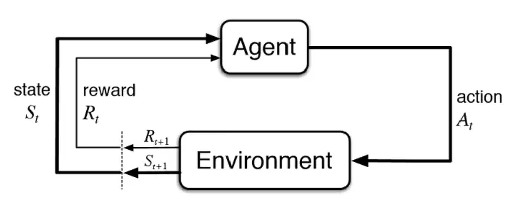
Figure: The agent–environment loop (illustration source: AltexSoft).

Two common approaches to learning behavior in this loop:

• Model-free RL learns a policy $\pi(a_t\mid \cdot)$ or a value function $Q(\cdot)$ directly from experience, without explicitly modeling the environment dynamics.
• Model-based RL additionally learns (or is given) an explicit environment model, something that predicts how the world changes—and uses it for planning, imagination, or to generate extra training data.

An influential template is Dyna: learn from real experience, learn/update a dynamics model, and do extra updates using model-generated rollouts (“simulated experience”). (Sutton & Barto, 2018)

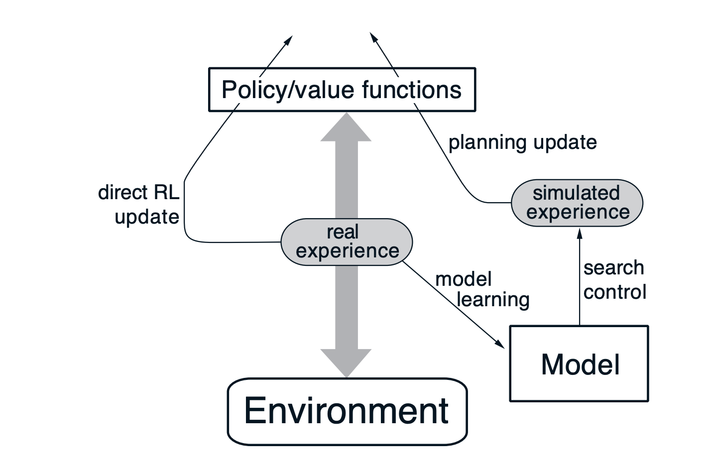
Figure: Dyna-style loop (real experience → model learning → simulated experience → planning update), adapted from Sutton & Barto, Reinforcement Learning: An Introduction. (Sutton & Barto, 2018)

This shows where “world models” live: a learned dynamics model the agent can query (for planning, imagination, or policy learning).

What exactly gets modeled?

In practice, a “world model” is defined less by a specific architecture and more by an interface: given what the agent has seen (and optionally what it does), the model produces a prediction of what comes next.

Across the literature, most differences boil down to a few recurring design choices that determine (i) what the model is asked to predict, (ii) whether it supports counterfactual interventions, and (iii) what kind of rollouts it can be used for.

Where do we model the world?

(a) Pixel / observation space. The most literal option is to predict next observations: \(p(x_{t+1}\mid x_{\le t}, a_{\le t})\) This is expressive and visually interpretable, but expensive and brittle: long-horizon rollouts tend to drift, and predicting every pixel forces the model to care about irrelevant details.

(b) Latent state space. Instead of predicting pixels, we encode observations into a compact latent state and predict dynamics there: \(x_t \xrightarrow{\text{encode}} s_t \xrightarrow{\text{predict}} s_{t+1}\) Latent modeling is the dominant recipe in “classic” model-based RL (PlaNet/Dreamer-style): it makes rollouts cheaper, supports planning/control more naturally, and often improves sample efficiency.

(c) Task-relevant / abstract space. Some approaches model only what is needed for decision making (e.g., reward/value/policy), without reconstructing the world visually. These “value-equivalent” models can be strong for planning, but may be harder to interpret as a simulator.

With or without action?

Action-conditioning is the difference between “prediction” and “counterfactual prediction.”

• Action-conditioned models aim to learn something like: \(p(x_{t+1}\mid x_{\le t}, a_t) \;\text{or}\; p(s_{t+1}\mid s_t, a_t)\) so the agent can ask: what happens if I do $a_t$?

• Action-free models (common in internet video pretraining and video generation) learn: \(p(x_{t+1}\mid x_{\le t})\) which can look like a “world simulator,” but lacks an explicit intervention handle. A large chunk of modern robotics work is about reintroducing an action channel (via post-training, latent actions, or interactive interfaces).

One-step causal vs whole-trajectory generation?

A subtle but important distinction:

• Online / causal world models are trained step-by-step $(t \to t+1)$ and naturally support rollouts.
• Offline / trajectory models (e.g., diffusion video generators) may generate an entire future clip at once. They can still be “world-model-like,” but the interface looks different.

In practice, stepwise models fit planning/control loops because they let you branch on candidate actions and replan; trajectory models are closer to open-loop generation unless you add an action-conditioned, closed-loop interface.

What are “world models”?

I’ll use the operational definition at the top of the post, but make it concrete with a unifying notation based on LeCun’s Enc/Pred scaffold (LeCun, 2024). This lets us organize the literature as variations in the choice of internal state $s_t$, where stochasticity enters (via $z_t$), whether the dynamics are action-conditioned, and the training objective.

I’ll keep notation consistent:

• Observation $x_t$ (image/video frame, proprioception, text token, etc.)
• Action $a_t$ (optional)
• Encoder $h_t = \mathrm{Enc}_\phi(x_t)$
• World-state $s_t$ (model’s internal state / belief)
• Stochastic latent $z_t \sim p_\theta(z_t \mid \cdot)$ (captures uncertainty / multimodality)
• Predictor $s_{t+1} = \mathrm{Pred}_\theta(h_t, s_t, a_t, z_t)$

A “world model” is then a learned transition model that supports counterfactual rollouts under proposed actions.

The unifying idea: learn a model of the environment, then use it to improve decision-making—often with much better sample-efficiency than purely model-free RL.

Latent dynamics: learned state-space models

The latent-dynamics line of work starts from a practical observation: predicting in raw pixel space is expensive and brittle, while predicting in a compact latent state can be both easier and more useful for control. The shared recipe is

\[x_t \xrightarrow{\mathrm{Enc}} s_t \xrightarrow{\mathrm{Pred}} s_{t+1}\]

where $s_t$ is a learned belief state (the agent’s internal state) that can be rolled forward under candidate actions.

A minimal formal template

A convenient abstraction for this family is a stochastic latent state-space model with an observation model and reward model:

\[\begin{aligned} h_t &= \mathrm{Enc}(x_t) \\ z_t &\sim p_\theta(z_t \mid s_t, a_t) \\ s_{t+1} &= f_\theta(s_t, a_t, z_t) \\ x_t &\sim p_\theta(x_t \mid s_t) \\ r_t &\sim p_\theta(r_t \mid s_t, a_t) \end{aligned}\]

Here $x_t$ denotes the observation (some papers write $o_t$). Intuitively:

• $h_t = \mathrm{Enc}(x_t)$: encode the current observation into a feature/latent used by the dynamics.
• $z_t \sim p_\theta(z_t\mid s_t,a_t)$: sample a stochastic “innovation” term (optional) to represent uncertainty/multimodal next states.
• $s_{t+1} = f_\theta(s_t,a_t,z_t)$: roll the internal state forward under the candidate action.
• $x_t \sim p_\theta(x_t\mid s_t)$: (optional) decode/reconstruct observations from state for representation learning and debugging.
• $r_t \sim p_\theta(r_t\mid s_t,a_t)$: (optional) predict reward (and often termination/discount) for planning/control.

Here $p_\theta(\cdot\mid\cdot)$ denotes learned conditional distributions parameterized by $\theta$; in practice these are neural heads that output distribution parameters (e.g., Gaussian moments or categorical logits).

Not every “world model” instantiates every head: Dreamer/PlaNet-style models usually learn both an observation decoder $p_\theta(x_t\mid s_t)$ and a reward model $p_\theta(r_t\mid s_t,a_t)$; MuZero-style models often skip pixel prediction entirely and instead model reward/value/policy in an abstract state.

Individual papers differ in how they parameterize $s_t$, where they place stochasticity, and how actions are selected from the model’s rollouts.

World Models (2018): explicit latents and explicit memory

World Models (Ha & Schmidhuber, 2018) is a canonical example of the “compress → predict → control” pattern: learn a latent simulator, then optimize a controller inside the model’s imagined rollouts. (Ha & Schmidhuber, 2018)

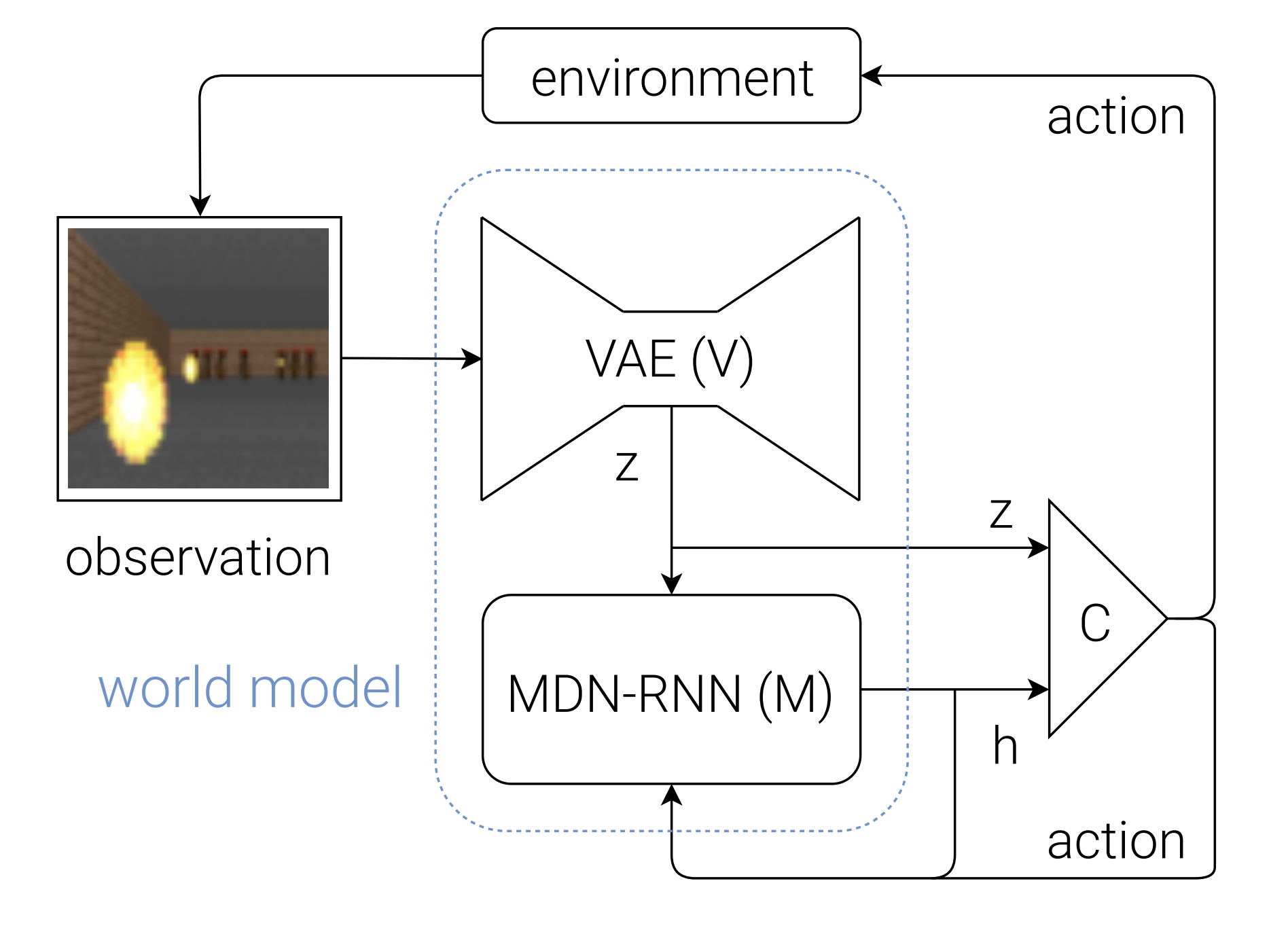
Figure: Overall architecture (VAE $\to$ MDN-RNN $\to$ controller) (source: Ha & Schmidhuber, 2018).

To keep notation consistent with the rest of this post, I’ll write observations as $x_t$ (the paper uses $o_t$). The model is modular:

• V (Vision, VAE) compresses each observation into a per-step latent $z_t$.
• M (Memory/dynamics, MDN-RNN) maintains a recurrent hidden state $h_t$ and predicts a distribution over the next latent.
• C (Controller) maps the current latent and memory to an action.

One way to write the core loop is:

\[\begin{aligned} z_t &= \mathrm{Enc}_\phi(x_t) \\ h_{t+1} &= \mathrm{RNN}_\theta(h_t, z_t, a_t) \\ z_{t+1} &\sim p_\theta\big(z_{t+1}\mid h_{t+1}\big) \\ a_t &= \mathrm{C}_\psi\big([z_t,\, h_t]\big) \end{aligned}\]

With abuse of notation, I’ll use $h_t$ here for the MDN-RNN hidden state (as in the original paper), even though earlier $h_t=\mathrm{Enc}(x_t)$ denoted encoder features in the generic template.

In this model, the dynamics component is trained to predict a conditional distribution over the next latent given action, current latent, and recurrent memory:

\[p_\theta\big(z_{t+1}\mid a_t, z_t, h_t\big) \quad\text{with}\quad h_{t+1}=\mathrm{RNN}_\theta(h_t, z_t, a_t),\]

implemented as a mixture-density head (MDN). At sampling time, a temperature parameter $\tau$ controls how stochastic the imagined rollouts are.

The original recipe is explicitly staged:

• Train the VAE on frames to learn \(\mathrm{Enc}_\phi\) (and a decoder for reconstruction/visualization), then encode trajectories into latents $z_{1:T}$.
• Train the MDN-RNN on latent sequences (with actions) by maximum likelihood: roll the RNN forward with teacher forcing and minimize the negative log-likelihood $-\log p_\theta(z_{t+1}\mid a_t, z_t, h_t)$.
• Optimize the controller parameters $\psi$ inside the learned model (in the paper: CMA-ES), using environment reward as the objective.

At inference / “dream rollout” time, the model is a simulator you can unroll: update the recurrent state deterministically, then sample the next latent from the MDN (temperature $\tau$ controls diversity):

\[h_{t+1} = \mathrm{RNN}_\theta(h_t, z_t, a_t), \qquad z_{t+1} \sim p_\theta(\cdot\mid h_{t+1}).\]

PlaNet: RSSM belief state and planning as action selection

PlaNet formalizes the latent-dynamics idea as a belief state-space model that is directly optimized for planning from pixels. The core object is a Recurrent State-Space Model (RSSM), where the internal state is a pair

\[s_t = (d_t, z_t)\]

with a deterministic memory component $d_t$ and a stochastic component $z_t$ that captures uncertainty and multimodality. The latent transition is typically written as

\[\begin{aligned} d_{t+1} &= g_\theta(d_t, z_t, a_t) \\ z_{t+1} &\sim p_\theta(z_{t+1}\mid d_{t+1}) \end{aligned}\]

and a learned posterior update (filter) incorporates the new observation:

\[z_{t+1} \sim q_\theta(z_{t+1}\mid d_{t+1}, x_{t+1}).\]

The details of the variational objective are not essential here. The important interface is that the model maintains a compact latent belief $s_t$ that can be rolled forward under candidate actions while remaining grounded in observations. (Hafner et al., 2019)

PlaNet explicitly learns a reward predictor in latent space, $\hat r_t = R_\theta(s_t, a_t)$, and uses it to score imagined trajectories. Action selection is performed by model predictive control (MPC): at each real environment step, PlaNet optimizes an open-loop action sequence of horizon $H$ by repeatedly rolling out the RSSM forward and maximizing predicted return:

\[\begin{aligned} a_{t:t+H-1}^* &= \arg\max_{a_{t:t+H-1}} \mathbb{E}\left[\sum_{k=0}^{H-1}\gamma^k\, R_\theta(s_{t+k}, a_{t+k})\right], \\ &\text{where}\quad s_{t+k+1} \sim p_\theta(\cdot \mid s_{t+k}, a_{t+k}). \end{aligned}\]

The expectation is over the model’s stochastic latents. In practice, PlaNet uses the cross-entropy method (CEM) to search over action sequences. After CEM returns an optimized sequence, the agent executes only the first action (a_t^*), receives the next observation, updates its belief state, and replans. This makes PlaNet a clear instance of an implicit policy: the planner is the policy. (Hafner et al., 2019)

Dreamer: imagination training and an explicit policy

Dreamer keeps the same high-level interface as PlaNet, a latent world model that can be rolled forward under actions, but it changes the control layer. PlaNet treats planning as the policy and solves an MPC problem at every step via CEM. Dreamer instead learns an explicit actor and critic using trajectories imagined inside the learned world model. The result is amortized control: at inference time, action selection is a single policy forward pass rather than an online optimization procedure. (Hafner et al., 2020)

Formally, let the world model define a stochastic latent transition \(s_{t+1} \sim p_\theta(\cdot \mid s_t, a_t), \qquad \hat r_t = R_\theta(s_t, a_t).\)

with $s_t$ an RSSM-style belief state. Dreamer introduces an actor $\pi_\psi(a_t\mid s_t)$ and a value function $V_\psi(s_t)$. The actor is trained to maximize predicted return under rollouts generated by the world model:

\[\max_\psi\; \mathbb{E}\left[\sum_{k=0}^{H-1}\gamma^k\, \hat r_{t+k}\right], \quad a_{t+k}\sim \pi_\psi(\cdot\mid s_{t+k}), \quad s_{t+k+1}\sim p_\theta(\cdot\mid s_{t+k}, a_{t+k}).\]

The critic provides value estimates and bootstrapping targets on imagined trajectories, allowing long-horizon learning without planning-time search at every environment step. Conceptually, the policy improvement step happens in the model’s latent “imagination,” rather than in the real environment. (Hafner et al., 2020)

JEPA: predict representations, not pixels

The key insight of Joint-Embedding Predictive Architectures (JEPA) is that a world model does not need to simulate every pixel to be useful. Instead, it should predict representations that capture the abstract structure of the world.

The architecture consists of three core components:

• Context Encoder: processes the observed part of the input (present) to produce a context representation.
• Target Encoder: processes the target part of the input (future or missing region) to produce the ground-truth representation.
• Predictor: takes the context representation and a condition (e.g., position or action) and predicts the target representation.

Crucially, there is no decoder back to pixels. The model is trained by matching the prediction to the target in embedding space. The main risk is representation collapse (e.g., the encoder outputting a constant vector), which is typically prevented by making the target encoder a slowly updating copy (EMA) of the context encoder.

I-JEPA: Image-based JEPA

I-JEPA instantiates this for images. The task is inpainting in latent space: given a visible context block of an image, predict the embeddings of masked target blocks.

I-JEPA in the unified notation

In terms of the notation used throughout this post:

• Input ($x$): The full image (or patches).
• Encoder ($h_t$): The Context Encoder maps visible patches $x_{\text{context}}$ to latent context $h = \mathrm{Enc}\theta(x{\text{context}})$.
• Target State ($s_t$): The Target Encoder maps the full image (or target regions) to semantic embeddings $s_{\text{target}} = \mathrm{Enc}{\bar\theta}(x{\text{target}})$.
• Condition ($z_t$): The conditioner is a set of positional mask tokens ${m_j}$ indicating where to predict.
• Predictor: A transformer that takes context and mask tokens to output predicted embeddings $\hat s$.

\[\hat s_{\text{target}} = \mathrm{Pred}_\phi(h, \{m_j\})\]

Architecture details

I-JEPA uses Vision Transformers (ViT) for all components, making the method scalable and efficient.

1. Targets: The input image $y$ is converted into patches and fed through the Target Encoder to obtain patch-level representations. Target blocks are sampled from these embeddings. The Target Encoder weights are updated via an exponential moving average (EMA) of the Context Encoder weights.
2. Context: A context block is sampled from the image, and any regions overlapping with the target blocks are removed. The Context Encoder processes only these visible patches.
3. Prediction: The Predictor is a narrow ViT. It takes the output of the Context Encoder and a set of learnable mask tokens with added positional embeddings corresponding to the target block locations. It outputs the predicted patch embeddings.
4. Loss: The model minimizes the average L2 distance between the predicted patch representations and the target patch representations:

\[\mathcal{L} = \frac{1}{M} \sum_{i=1}^M \sum_{j \in B_i} \left\| \hat s_j^{(i)} - \mathrm{StopGrad}(s_j^{(i)}) \right\|_2^2\]

By predicting high-level representations of missing regions rather than pixel values, I-JEPA learns semantic features that abstract away unnecessary low-level details. (Assran et al., 2023)

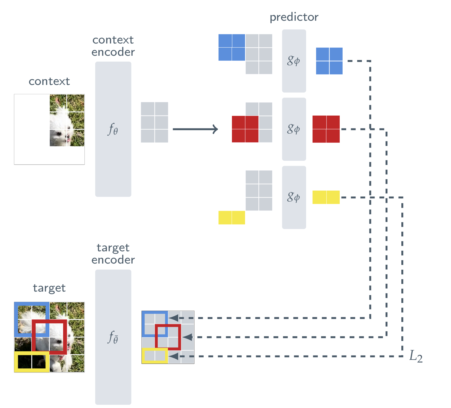
Figure: I-JEPA architecture (Assran et al., 2023). The model uses a single context block to predict representations of multiple target blocks from the same image. The Context Encoder (ViT) processes only visible patches. The Predictor (narrow ViT) uses the context output and positional mask tokens to predict target representations. These targets are generated by a Target Encoder, updated via exponential moving average (EMA) of the context encoder. (Assran et al., 2023)

V-JEPA: from images to video

V-JEPA extends the Joint-Embedding Predictive Architecture to video. The objective is spatiotemporal mask-denoising in representation space: predicting the embeddings of missing “tubelets” (3D video patches) from the visible parts of the video.

Key differences from I-JEPA

While the high-level components (Context Encoder, Target Encoder, Predictor) remain the same, V-JEPA makes critical changes to handle time and scale:

1. Tubelet Tokenization: Instead of flat 2D patches, the video is patchified into tubelets of size $T \times H \times W$ (e.g., $2 \times 16 \times 16$). This captures local motion immediately at the input level.
2. 3D Rotary Position Embeddings (RoPE): To better encode relative positions in space and time, modern versions (V-JEPA 2) replace absolute embeddings with 3D-RoPE. The feature embedding is split into three segments, with rotations applied separately for time, height, and width.
3. L1 Loss: The model minimizes the L1 distance between predictions and targets (unlike the L2 loss common in I-JEPA):

\[\mathcal{L} = \| \mathrm{Pred}_\phi(h, \{m_j\}) - \mathrm{StopGrad}(s_{\text{target}}) \|_1\]

Scaling to a foundation model

The effectiveness of V-JEPA depends heavily on scale. The V-JEPA 2 recipe involves scaling to 22 million videos and 1 billion parameters (ViT-g), and using a training curriculum that starts with lower-resolution clips and increases resolution/length over time. (Bardes et al., 2025)

V-JEPA 2: from video foundation to physical planning

V-JEPA 2 demonstrates how to turn a passive video foundation model into a physical world model. The strategy splits learning into two phases: large-scale action-free pretraining (learning independent physics) and small-scale action-conditioned adaptation (learning control).

1. Action-free pretraining (V-JEPA): Train a large ViT-g encoder on 22M passive videos using the standard mask-denoising objective.
2. Action-conditioned adaptation (V-JEPA 2-AC): Freeze the encoder and learn a lightweight predictor on a smaller robotics dataset (e.g., Droid, end-effector control).

V-JEPA 2-AC: making V-JEPA controllable

Action-free V-JEPA is a strong predictive prior, but it does not directly incorporate the causal effect of actions. V-JEPA 2-AC adds an action-conditioned predictor on top of the frozen foundation encoder, trained on a small amount of interaction data.

Concretely, the pre-trained video encoder is kept frozen and used as a per-frame image encoder:

\[s_t := \mathrm{Enc}_{\text{fixed}}(x_t)\]

(The V-JEPA 2 paper writes these feature maps as $z_t$.) The action-conditioned predictor then learns dynamics over these states.

• Inputs: an interleaved sequence of encoded frames $s_t$, robot proprioceptive state $p_t$ (end-effector pose), and actions $a_t$.
• Predictor: a block-causal transformer that predicts the next representation $\hat s_{t+1}$.
• Training loss: L1 in representation space, mixing teacher forcing and short rollouts to reduce error accumulation:

\[\mathcal{L}(\phi) = \underbrace{\sum_{t} \|\hat s_{t+1} - s_{t+1}\|_1}_{\text{teacher forcing}} + \underbrace{\|\mathrm{Rollout}_\phi(s_1, p_1, a_{1:H}) - s_{H+1}\|_1}_{\text{rollout loss}}\]

V-JEPA 2-AC in the unified notation

With the notation used throughout this post, the learned transition is:

\[\hat s_{t+1} = \mathrm{Pred}_\phi\big(s_{\le t},\, p_{\le t},\, a_{\le t}\big), \qquad s_t = \mathrm{Enc}_{\text{fixed}}(x_t)\]

There is still no pixel decoder; the internal state is the encoder’s embedding. This is enough to support goal-conditioned planning by searching over action sequences that make the predicted future representation match the goal representation $s_g=\mathrm{Enc}_{\text{fixed}}(x_g)$:

\[a^*_{1:T} = \arg\min_{a_{1:T}} \left\|\mathrm{Rollout}_\phi(s_t, p_t, a_{1:T}) - s_g\right\|_1.\]

So the conceptual step from V-JEPA to V-JEPA 2-AC is: masked representation prediction $\rightarrow$ action-conditioned latent rollouts usable inside MPC. (Bardes et al., 2025)

This gives a compact way to relate JEPA to generative latent-dynamics models: Dreamer-like methods keep latents grounded by making them predictive of $x_t$ through an observation model; JEPA-like methods remove the decoder and instead pay an explicit “anti-collapse” tax (EMA target encoder). The resulting representation may be less tied to pixel-level detail, but it can be easier to scale and can serve as a strong prior for downstream planning when an action-conditioned head is introduced. (Assran et al., 2023; Bardes et al., 2025)

Video foundation models and interactive world models

Internet-scale video generation reopened the “world model” conversation because the samples often look like simulation: object permanence, stable scenes, plausible interactions, and long-range coherence. But in the RL sense used earlier, visual plausibility is not the same as a world model. A video generator can be an excellent model of the distribution of videos people upload to the internet, while still lacking the core interface an agent needs for counterfactual reasoning under interventions. (OpenAI)

A useful way to formalize this difference is to separate trajectory models from action-conditioned transition models. Many video generators are best written as modeling a joint distribution over entire trajectories:

\[p_\theta(x_{1:T}\mid c)\]

where $c$ is prompt context such as text, an image, or a few conditioning frames. This is not the same object as an environment model used in RL, which needs an explicit action channel:

\[p_\theta(x_{t+1}\mid x_{\le t}, a_t)\]

or, in latent form,

\[s_{t+1} = \mathrm{Pred}(s_t, a_t, z_t), \qquad x_{t+1}\sim p(x_{t+1}\mid s_{t+1})\]

The key distinction is whether $a_t$ is a first-class input with consistent semantics across time, so the model answers “what happens if I do this now?” rather than “what continuation is plausible given this prompt?”

This also clarifies how to map video generators into the Enc/Pred/Dec scaffold without committing to the label “world model.” Many modern systems look like:

\(h = \mathrm{Enc}(x_{1:k}) \quad (\text{tokenizer / latent encoder})\) \(\tilde h_{1:T} = \mathrm{Pred}(h, z) \quad (\text{trajectory generator, often diffusion or AR})\) \(x_{1:T} = \mathrm{Dec}(\tilde h_{1:T})\)

This is a powerful generative modeling pipeline, but it becomes “world-model-like” only when it supports iterative online updates and action-conditioned counterfactuals.

Plausibility vs counterfactual control

The practical critique can be stated in one sentence: a convincing video continuation does not imply reliable counterfactual control. RL-style world models require that interventions cause consistent downstream changes. In notation, the requirement is not “can it sample plausible $x_{1:T}$?” but “given the same state $s_t$, do different actions $a_t$ produce different, consistent futures according to $\mathrm{Pred}(s_t, a_t, z_t)$?” This is why action-free pretraining can be an excellent prior, but it is not sufficient to claim an environment model.

Genie (1/2/3): when the action channel arrives

The Genie line is a good organizing example because it explicitly aims at interactive generation, meaning the model is queried online and responds to actions step-by-step.

Genie (the 2024 paper) is presented as a “generative interactive environment” trained from unlabeled internet videos. Its key ingredients are a spatiotemporal video tokenizer, an autoregressive dynamics model, and a latent action model that enables users to act frame-by-frame despite the lack of action labels during training. That last part matters: Genie is explicitly trying to introduce an action interface into a model trained largely from passive observations. (Bruce et al., 2024)

Genie 2 is framed as a larger-scale foundation world model that can generate a diverse set of 3D-like interactive worlds and simulate the consequences of actions such as movement and interaction. The emphasis is still the same interface shift: the model is no longer just producing a trajectory conditioned on a prompt, it is maintaining something like an internal state that updates online under user actions. (Google DeepMind)

Genie 3 pushes further in the same direction and emphasizes real-time interactive generation (reported as 24 FPS at 720p in external reporting) and longer interaction horizons. In the terms of this post, Genie 3 is “world-model-like” primarily because it makes the counterfactual query feel operational: “go left” is a well-defined action input repeatedly applied over time, not a one-shot conditioning prompt. (Google DeepMind, 2025)

A compact way to summarize Genie 1/2/3 as a single arc is: start from passive video priors, add an action interface via latent actions and interactive rollouts, then extend coherence and controllability as the primary product requirement. The underlying modeling choices can vary, but the contribution is consistent: Genie treats interactivity as part of the definition, not a downstream add-on.

Cosmos: the “Physical AI platform” view of world models

Cosmos is useful here because it explicitly targets the bridge from video priors to physical AI workflows. Rather than positioning “world model” as a single monolithic model, Cosmos frames a platform: video curation, video tokenizers, pretrained world foundation models, and post-training recipes to adapt a general world model into a setup-specific simulator for robotics or autonomous driving. (NVIDIA, 2025)

Two points connect Cosmos cleanly to the formalism in earlier sections:

• Cosmos treats a world foundation model as a general-purpose prior that can be fine-tuned into a customized environment model. This matches the idea that passive video can give you strong dynamics priors, but you still need alignment to actions, sensors, and downstream objectives for control. (NVIDIA, 2025)
• Cosmos explicitly describes the “digital twin” framing: a policy model, and a world model that can generate the training data and scenarios needed before real-world deployment. This makes the role of world models concrete as infrastructure for Physical AI, not just a benchmark agent component. (NVIDIA, 2025)

Where this sits relative to latent-dynamics and JEPA

PlaNet and Dreamer start from interaction data and build a compact belief state that is immediately usable for counterfactual rollouts under $a_t$. JEPA starts with representation prediction and adds action-conditioning later (for example via an action-conditioned variant). Video foundation models contribute a different strength: they give a broad prior over dynamics and appearance from passive data. Whether they become world models in the RL sense depends on whether an action channel is learned, made explicit, and kept consistent over online rollouts.

From world model to robot policy

Robotics is the hard test

Robotics forces “world model” to mean counterfactual, action-conditioned prediction. In video generation, it can be enough that samples look plausible under a prompt distribution. In robotics, the model is repeatedly queried while the agent intervenes, so three requirements become non-negotiable:

• an explicit action channel $a_t$ whose semantics are stable over time
• a stable internal state $s_t$ that does not drift as rollouts get longer
• rollouts that remain useful under distribution shift, since the policy will visit states the dataset undersampled

In the notation used throughout this post, robotics asks for a transition interface of the form

\[s_{t+1}=\mathrm{Pred}(h_t,s_t,a_t,z_t), \qquad h_t=\mathrm{Enc}(x_t)\]

where $z_t$ captures uncertainty and multimodality, and where the model remains meaningful when the policy proposes new actions.

The controllability gap

Internet-scale pretraining can produce a powerful predictor of what tends to happen next, but passive video typically supports objectives closer to

\[p(x_{t+1}\mid x_{\le t})\]

not the interventional object needed for control

\[p(x_{t+1}\mid x_{\le t}, a_t)\]

This gap is the main reason “video realism” does not automatically translate into robotics competence. The missing piece is not only an action token, but an action variable that is grounded in the world model’s state update. In practice, robotics adaptation becomes a concrete question:

where does $a_t$ come from, and how is it represented so that $\mathrm{Pred}$ produces consistent counterfactual rollouts?

This is exactly the role played by latent actions, inverse dynamics, action tokenizers, and post-training pipelines that inject an action channel into an otherwise passive predictor.

AdaWorld: latent actions as a universal action interface

AdaWorld is a clean exemplar of one answer: introduce a latent action $u_t$ as an intermediate interface that makes passive transitions “interactive.” The high-level idea is to learn a world model whose dynamics are conditioned on $u_t$, where $u_t$ is inferred from state transitions even when the true low-level action space is unknown, heterogeneous, or changes across environments. (AdaWorld, 2025)

A concise formulation in the unified notation is:

\(h_t=\mathrm{Enc}(x_t)\) \(u_t \sim q_\phi(u_t \mid x_t, x_{t+1})\) \(s_{t+1}=\mathrm{Pred}_\theta(h_t,s_t,u_t,z_t)\)

The latent action $u_t$ plays the role of a control token that “explains” why the world moved from $x_t$ to $x_{t+1}$. Once the model is trained, control can happen in the $u$-space even if the downstream environment exposes a different concrete action space. AdaWorld’s adaptation story is then:

• keep the learned latent action dynamics fixed
• learn a small adapter that maps real actions $a_t$ in a new environment to latent actions $u_t$, or learn a policy that outputs $u_t$ directly
• use the world model’s rollouts in latent action space for planning or policy learning

This makes the “action channel” portable: $u_t$ becomes a universal interface that can be reused across environments with different physical action parameterizations. (AdaWorld, 2025)

Why latent actions help

Latent actions complete the RL loop for passive predictors by turning “what happens next” into “what happens if I do this.” The coupling to policy learning can be expressed in two equivalent ways that match the earlier policy axis.

An explicit policy over latent actions:

\(u_t \sim \pi_\psi(\cdot\mid s_t)\) \(s_{t+1}\sim p_\theta(\cdot\mid s_t,u_t)\)

Or an implicit policy by planning in latent action space:

\[u_{t:t+H-1}^*=\arg\max_{u_{t:t+H-1}} \mathbb{E}\Big[\sum_{k=0}^{H-1}\gamma^k \hat r_{t+k}\Big]\]

where imagined rewards $\hat r_{t+k}$ are predicted from the rolled state, and the expectation is over $z_t$.

The final step is grounding back to the robot:

• either decode $u_t \rightarrow a_t$ through an adapter learned from demonstrations or interaction
• or treat $u_t$ as the control signal directly if the actuator interface is learned end-to-end

This is the conceptual bridge: latent actions turn passive prediction into interactive modeling. They provide an $a_t$-like variable that the world model can condition on, without requiring the action space to be fixed across domains.

Relation to Cosmos Policy

AdaWorld and Cosmos Policy attack the same bottleneck, connecting rich predictive priors to control, but from opposite directions.

AdaWorld creates interactivity by learning an action representation $u_t$ from observed transitions and then adapting this action interface across environments. (AdaWorld, 2025)

Cosmos Policy starts with a large pretrained video model and post-trains it into a robot policy by directly generating actions inside the model’s latent diffusion process. It also predicts future states and values to enable test-time planning via sampling and ranking. (NVIDIA, 2026)

A compact way to say it is:

• AdaWorld emphasizes a transferable action interface $u_t$ and small adapters for new action spaces.
• Cosmos Policy emphasizes a post-training recipe that turns a video foundation model into a direct visuomotor policy, optionally augmented with model-based planning via future prediction and value estimation. (NVIDIA, 2026)

Other routes to add actions

AdaWorld is one clean exemplar, but it is not the only pattern for introducing an action variable.

• Inverse dynamics models infer an action-like variable from ((x_t,x_{t+1})), then use it for forward dynamics or policy learning.
• Unified video–action latents learn shared representations that support both future prediction and action decoding.
• Geometric or flow-based intermediates replace pixel prediction with structured motion targets such as point tracks or mask flow, which can serve as a controllable planning interface for manipulation. (Track2Act, 2024; Mask2Act, 2025)

The common theme is the same: robotics demands an explicit intervention channel. Different methods disagree on whether that channel should be the robot’s native action ($a_t$), a learned latent action ($u_t$), or a structured motion interface, but all of them are ways of making $\mathrm{Pred}$ answer counterfactual questions rather than passive continuations.

Limits, evaluation, and what to watch next

Evaluation: what would prove “world model” in the RL sense? The bar is not photorealistic samples; it’s whether a model supports reliable intervention. Three practical criteria are: (i) counterfactual control (changing $a_t$ changes predicted outcomes in consistent ways), (ii) long-horizon consistency under interventions (closed-loop rollouts don’t quickly drift when the agent replans and acts), and (iii) downstream planning success (using the model inside MPC or as a training signal measurably improves task performance).

Failure modes. The usual pitfalls are exactly the ones that make model-based RL hard: compounding error in rollouts, brittleness under out-of-distribution actions/states, and “physics-looking” predictions that are correlation-driven rather than causal. If you also learn rewards or values, you inherit another class of issues: models can become miscalibrated and planning can exploit reward/value errors (a form of reward hacking).

Where the field is converging. There’s a visible two-track convergence: better internal representations (JEPA-style objectives, structured state, and more explicit geometry) and better generative priors (scaled video diffusion / autoregressive models). The bridge between them is action alignment: taking strong passive predictors and post-training them on interaction data (or learning latent-action interfaces) so the model can be used for counterfactual rollouts.

Future bets. The near-term product bets look less like one magic architecture and more like stacking the pieces that make models usable in the loop:

• physics-aware video priors adapted to control (robot post-training, MPC-style planning)
• 3D / spatial representations as a first-class internal state (not just pixels)
• evaluation shifting from “nice videos” to closed-loop task success and robustness